Parler Quick Ad-hoc Analysis

Published on Tuesday, 16 February, 2021 general

Parler Data Analysis

https://towardsdatascience.com/visualizing-geospatial-data-in-python-e070374fe621 https://mode.com/blog/python-data-visualization-libraries/

python !mkdir data

python !ls -n

total 24
-rw-r--r-- 1 1000 100 18504 Nov 13 21:01 change_detection.ipynb
drwxr-xr-x 2 1000 100    64 Feb 18 00:34 data
-rw-r--r-- 1 1000 100    72 Feb 18 00:33 parler_data.ipynb

python !curl -LOk https://srv-store6.gofile.io/download/7Wg83o/parler-videos-geocoded.csv.zip > data/parler-videos-geocoded.csv.zip

  % Total    % Received % Xferd  Average Speed   Time    Time     Time  Current
                                 Dload  Upload   Total   Spent    Left  Speed
100 1371k  100 1371k    0     0  71794      0  0:00:19  0:00:19 --:--:--  179k

python !cd data;ls -n

total 3340
-rw-r--r-- 1 1000 100 3416205 Jan 12 05:54 parler-videos-geocoded.csv
-rw-r--r-- 1 1000 100       0 Feb 18 00:41 parler-videos-geocoded.csv.zip

python import pandas as pd

python df = pd.read_csv('data/parler-videos-geocoded.csv')

python df.head(5)

	Longitude	Latitude	Timestamp	ID
0	0.0000	0.0000	2010-08-08 21:44:38	PtowPIzpewhu
1	0.0000	0.0000	2011-03-19 16:48:35	dGOhNqNgNywF
2	-118.8878	39.5554	2011-08-01 22:22:40	RGTLwBQugFNU
3	-74.6049	39.3308	2011-11-11 21:36:54	YNBV5GZkeM2E
4	-101.8747	33.4269	2012-12-24 22:50:15	oqLyjjYghOMi

python df.dtypes

Longitude    float64
Latitude     float64
Timestamp     object
ID            object
dtype: object

python df['Timestamp']=pd.to_datetime(df['Timestamp'])

python df['Timestamp'].min()

Timestamp('2010-08-08 21:44:38')

python df['Timestamp'].max()

Timestamp('2021-01-10 14:30:29')

python def years(x): return x.strftime('%Y-%m')

python df['YYYY-MM']=df['Timestamp'].apply(lambda x: years(x))

python timeseries=pd.DataFrame(df.groupby('YYYY-MM').count()['ID']) timeseries.tail(5)

	ID
YYYY-MM
2020-09	4127
2020-10	6107
2020-11	23634
2020-12	11452
2021-01	5988

```python

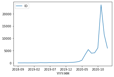
Parler launched September 2018

t = timeseries[timeseries.index>='2018-09'] ```

python t.plot()

<AxesSubplot:xlabel='YYYY-MM'>

png

```python import numpy as np import matplotlib.pyplot as plt

plt.figure(figsize=(20, 12))

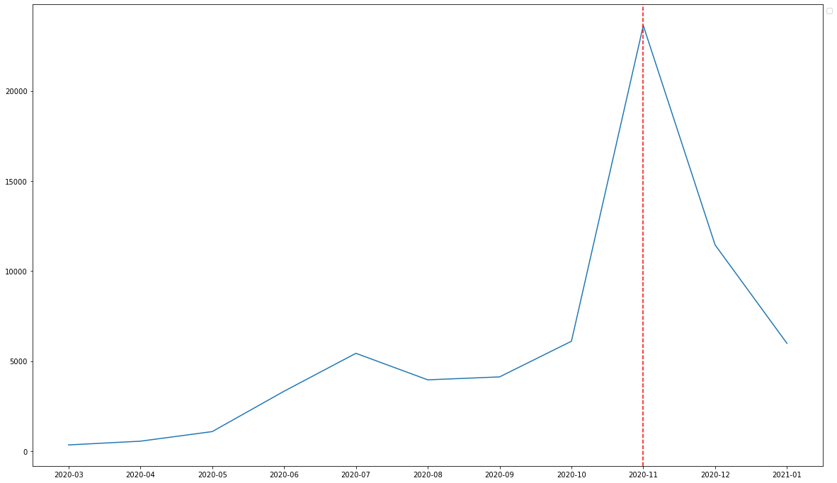
t2 = timeseries[timeseries.index>='2020-03']

only one line may be specified; full height

plt.axvline(x=36, color='b', label='axvline - full height')

place legend outside

plt.legend(bbox_to_anchor=(1.0, 1), loc='upper left') plt.plot(t2.index,t2['ID']) plt.axvline(x='2020-11', color='r', label='axvline - partial height',ls='--') plt.show() ```

No handles with labels found to put in legend.

png

```python

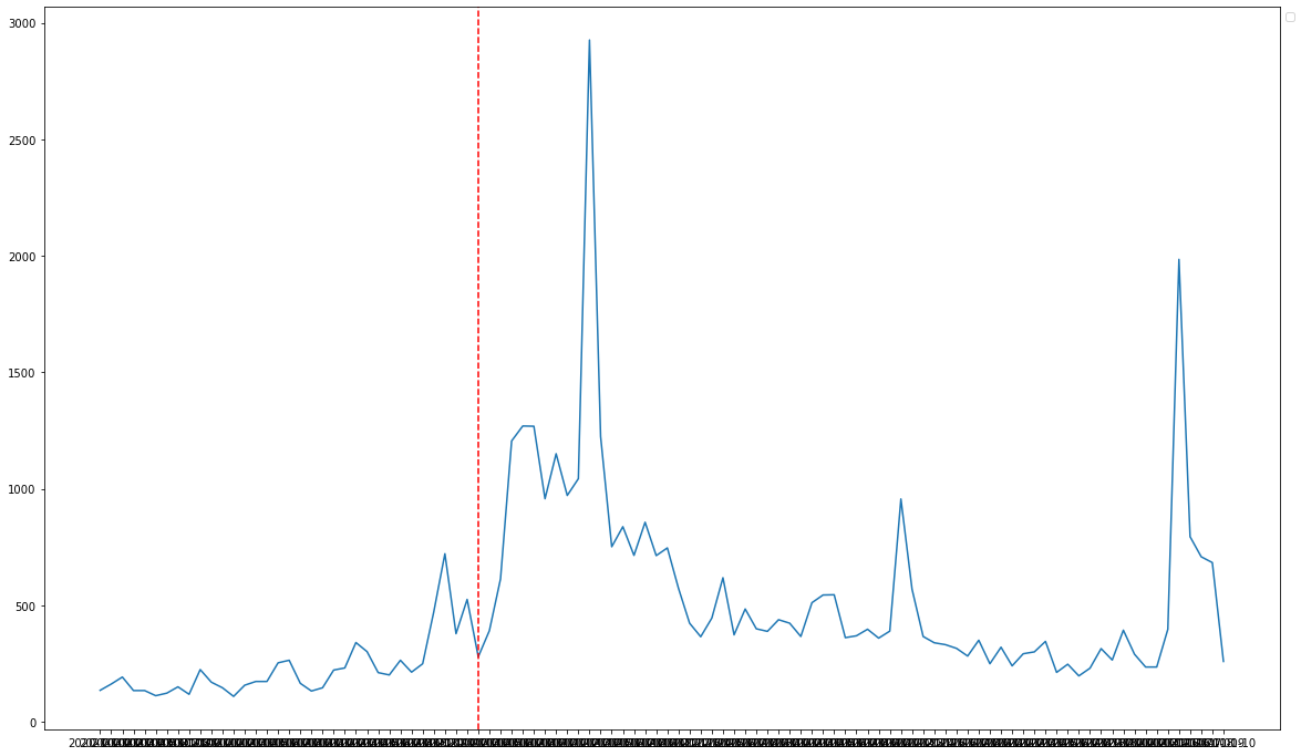
adding back day to chart out twitter suspensions

def days(x): return x.strftime('%Y-%m-%d')

df['day']=df['Timestamp'].apply(lambda x: days(x)) t2 = pd.DataFrame(df.groupby('day').count()['ID']) t2 = t2[t2.index>='2020-10'] ```

python t2[t2.index>'2020-01-01']

	ID
day
2020-10-01	136
2020-10-02	163
2020-10-03	193
2020-10-04	135
2020-10-05	135
...	...
2021-01-06	1985
2021-01-07	795
2021-01-08	709
2021-01-09	684
2021-01-10	260

102 rows × 1 columns

```python from matplotlib.dates import DateFormatter t2

plt.figure(figsize=(20, 12)) plt.legend(bbox_to_anchor=(1.0, 1), loc='upper left') plt.plot(t2.index,t2['ID']) plt.axvline(x='2020-11-04', color='r', label='axvline - partial height',ls='--')

plt.xticks(rotation=17,3)

plt.show() ```

No handles with labels found to put in legend.

png

```python plt.figure(figsize=(10, 7))

t2 = timeseries[timeseries.index>='2020-03']

only one line may be specified; full height

plt.axvline(x=36, color='b', label='axvline - full height')

place legend outside

plt.legend(bbox_to_anchor=(1.0, 1), loc='upper left') plt.plot(t2.index,t2['ID']) plt.axvline(x='2020-11', color='r', label='axvline - partial height',ls='--') plt.show() ```

```python import numpy as np

import matplotlib.image as mpimg from mpl_toolkits.basemap import Basemap

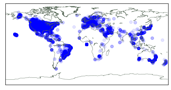
fig, ax = plt.subplots() earth = Basemap(ax=ax) earth.drawcoastlines(color='#556655', linewidth=0.5) ax.scatter(df['Longitude'],df['Latitude'],c='blue',alpha=0.1) ```

<matplotlib.collections.PathCollection at 0x7f7384bd3460>

png

```python

Make the figure

fig = plt.figure() ax = fig.add_subplot(111)

Map of Washington, DC

bot_left_lat =38.808277 bot_left_lon =-76.914339 top_right_lat =38.978921 top_right_lon = -77.140698

create the map object, m

m = Basemap(resolution='f', projection='cyl', \ llcrnrlon=bot_left_lon, llcrnrlat=bot_left_lat, \ urcrnrlon=top_right_lon, urcrnrlat=top_right_lat,ax=ax)

m.drawstates() ax.scatter(df['Longitude'],df['Latitude'],c='blue',alpha=0.1) ```

<matplotlib.collections.PathCollection at 0x7f7385005f10>

png

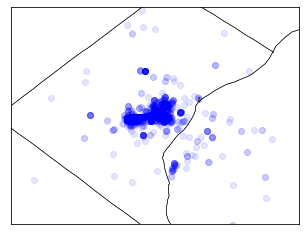
dc area

top,left = [38.978921, -77.140698] bottom,right = [38.808277, -76.914339]

Not very interesting

```python import conda import os

conda_file_dir = conda.file conda_dir = conda_file_dir.split('lib')[0] proj_lib = os.path.join(os.path.join(conda_dir, 'share'), 'proj') os.environ["PROJ_LIB"] = proj_lib ```

```python

```

```python

```