Galton-Watson Process

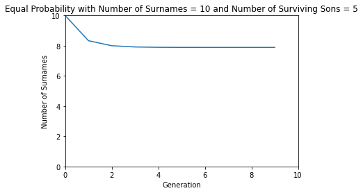
This study of the Galton-Watson Process, a branching process, solves problems around the development of a population under certain conditions. Galton originally proposed a mathematical question regarding the distribution of surnames in an idealized population.

Let $(Z_n)_n\geq0$ be a sequence of integer-valued random variables defined by

$\large \Zeta_n = \sum_{k=1}^{Z_n} X_n,_k, n \geq 1$

where ${X_n,_k : n,k \in \N}$​ forms a family of of independent and identically distributed natural-valued random variables.

The extinction probablity is given by

$lim P_i(Z_n=0)$

The Code

import matplotlib.pyplot as plt
from scipy.stats import poisson
from functools import reduce
from numpy.polynomial import Polynomial

def compose(fn, x, n):
    return reduce(lambda res, func: func(res), [fn] * n, x)

def equal_probability():
    number_of_surnames = 10
    number_of_surviving_sons = 5
    number_of_generations = 10
    fn = Polynomial([1 / (number_of_surviving_sons + 1)] * (number_of_surviving_sons + 1))
    plot_graph(fn,
               number_of_surnames,
               number_of_generations,
               "Equal Probability with Number of Surnames = {0} and Number of Surviving    Sons = {1}".format(number_of_surnames, number_of_surviving_sons))

def varying_likelihood():
    number_of_surnames = 10
    number_of_surviving_sons = 5
    number_of_generations = 10

    chance_of_i_surviving_sons = [1 / (number_of_surviving_sons + i) for i in range(1, number_of_surviving_sons + 1)]
    chance_of_0_surviving_sons = 1 - sum(chance_of_i_surviving_sons)

    fn = Polynomial([chance_of_0_surviving_sons] + chance_of_i_surviving_sons)

    plot_graph(fn,
               number_of_surnames,
               number_of_generations,
               "Varying Likelyhood with Number of Surnames = {0} and Number of Surviving Sons = {1}".format(
                   number_of_surnames, number_of_surviving_sons)
               )

def poisson_distribution():
    number_of_surnames = 10
    number_of_surviving_sons = 5
    mean_number_of_surviving_sons = 1
    number_of_generations = 10

    chance_of_i_surviving_sons = [
        poisson.pmf(i, mean_number_of_surviving_sons) for i in range(0, number_of_surviving_sons + 1)
    ]

    fn = Polynomial(chance_of_i_surviving_sons)

    plot_graph(fn,
               number_of_surnames,
               number_of_generations,
               "Poisson Distribution with Number of Surnames = {0} and Number of Surviving Sons = {1}".format(
                   number_of_surnames, number_of_surviving_sons)
               )

def plot_graph(fn, number_of_surnames, number_of_generations, title):
    generating_functions = [compose(fn, 0, generation) for generation in range(0, number_of_generations)]

    points = [number_of_surnames - number_of_surnames * func for func in generating_functions]

    plt.plot(points)
    plt.xlabel('Generation')
    plt.ylabel('Number of Surnames')
    plt.title(title)
    plt.axis([0, number_of_generations, 0, number_of_surnames])
    plt.show()


​    
equal_probability()
varying_likelihood()
poisson_distribution()

Let's simulate South Korean surnames to see which surnames are likely to die out in $nth$ generation.

Korean Surnames

References:

Galton-Watson Process Wikipedia